Mathematical Properties of Brownian Motion: A Visual Guide
This post provides the mathematical foundation for understanding Brownian Motion and Modern Generative Models. It can be read independently or as a prerequisite for that post.
Table of Contents
- Introduction
- The Four Defining Properties
- Visual Exploration
- Key Mathematical Properties
- The Wiener Process Construction
- Why These Properties Matter
- Mathematical Implications
- Connection to Diffusion Models
- Further Reading
Introduction
Brownian motion, named after botanist Robert Brown’s 1827 observation of pollen grains jittering in water, is one of the most important stochastic processes in mathematics. Formally known as the Wiener process after Norbert Wiener’s rigorous mathematical construction in 1923, it serves as the foundation for:
- Stochastic calculus (Itô calculus)
- Financial mathematics (Black-Scholes model)
- Physics (thermal fluctuations, diffusion)
- Machine learning (diffusion models, score-based generative models)
This post explores the mathematical properties that make Brownian motion so special, with visualizations to build intuition.
The Four Defining Properties
A standard Brownian motion (or Wiener process) $W(t)$ is a continuous-time stochastic process uniquely characterized by four properties:
Property 1: Starting from Zero
\[W(0) = 0 \quad \text{with probability 1}\]Meaning: Every Brownian motion path begins at the origin. This is a normalization convention—we can always shift a Brownian motion to start elsewhere.
Why it matters: Provides a fixed reference point for measuring displacement. In physics, this represents starting from a known initial position.
Property 2: Independent Increments
For non-overlapping time intervals $[t_1, t_2]$ and $[t_3, t_4]$ where $t_2 \leq t_3$:
\[W(t_2) - W(t_1) \text{ is independent of } W(t_4) - W(t_3)\]Meaning: What happens in one time interval doesn’t affect what happens in a non-overlapping interval. The process has “no memory” between disjoint time periods.
Example: If a particle moves 2 units right between $t=0$ and $t=1$, this tells us nothing about whether it will move left or right between $t=3$ and $t=4$.
Why it matters: Crucial for mathematical tractability. Allows us to analyze the process in segments and combine results.
Property 3: Stationary Gaussian Increments
For any $s < t$:
\[W(t) - W(s) \sim \mathcal{N}(0, t - s)\]Meaning:
- Stationary: The distribution depends only on the time difference $(t-s)$, not on absolute time
- Gaussian: The increment follows a normal distribution
- Variance grows linearly: $\text{Var}[W(t) - W(s)] = t - s$
Implications:
- $\mathbb{E}[W(t) - W(s)] = 0$ (zero drift on average)
- Longer time intervals → larger variance → more spread
- Since $W(0) = 0$, we have $W(t) \sim \mathcal{N}(0, t)$
Why it matters: Gaussian distributions are mathematically tractable and arise naturally from the Central Limit Theorem (sum of many small random shocks).
Property 4: Continuous Paths
\[W(t) \text{ is continuous in } t \text{ (almost surely)}\]Meaning: Brownian motion paths are continuous functions of time—no jumps or discontinuities. You can draw the path without lifting your pen.
Counterintuitive fact: Despite being continuous, Brownian motion is nowhere differentiable with probability 1. The paths are infinitely “jagged.”
Why it matters: Distinguishes Brownian motion from jump processes (like Poisson processes). Continuity is essential for Itô calculus.
Visual Exploration
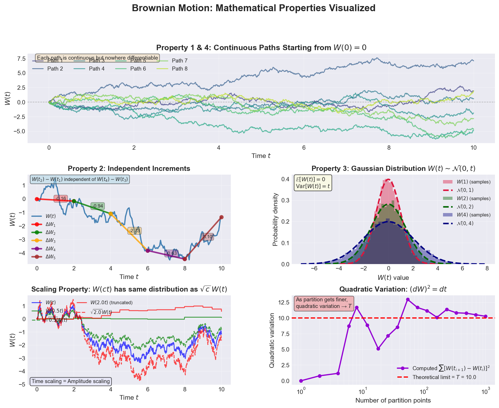
Figure: Comprehensive visualization of Brownian motion’s mathematical properties. The five panels demonstrate: (1) multiple continuous paths starting from zero, (2) independent increments over non-overlapping intervals, (3) Gaussian distribution of values at different times with variance increasing linearly, (4) scaling property showing equivalence between time-scaling and amplitude-scaling, and (5) quadratic variation converging to T as the partition becomes finer.
Panel Interpretations
Top Panel - Continuous Paths:
- 8 different realizations of Brownian motion
- All start at $W(0) = 0$
- Each follows its own random trajectory
- Notice the “roughness”—paths change direction constantly
Middle Left - Independent Increments:
- Single Brownian path with highlighted segments
- Each colored segment represents $\Delta W_i = W(t_{i+1}) - W(t_i)$
- The numerical values show the increments
- These increments are statistically independent
Middle Right - Gaussian Distribution:
- Histograms show empirical distribution of $W(t)$ at three times
- Overlaid curves show theoretical $\mathcal{N}(0, t)$ distributions
- Notice how variance increases with time: $\sigma^2 = t$
- Perfect match validates the Gaussian increment property
Bottom Left - Scaling Property:
- Demonstrates self-similarity: $W(ct) \stackrel{d}{=} \sqrt{c} \, W(t)$
- Time-scaled paths (solid lines) match amplitude-scaled paths (dashed lines)
- Fundamental to understanding diffusion at different scales
Bottom Right - Quadratic Variation:
- Shows $\sum [W(t_{i+1}) - W(t_i)]^2$ for increasingly fine partitions
- Converges to $T$ (the time horizon)
- This is the mathematical foundation of Itô calculus: $(dW)^2 = dt$
Key Mathematical Properties
Scaling Property
\[W(ct) \stackrel{d}{=} \sqrt{c} \, W(t) \quad \text{for any } c > 0\]Proof sketch:
- Left side: $W(ct) - W(0) = W(ct) \sim \mathcal{N}(0, ct)$
- Right side: $\sqrt{c} \, W(t) \sim \mathcal{N}(0, c \cdot t)$
- Both have the same distribution!
Physical interpretation: Brownian motion looks statistically the same at different time scales, just stretched or compressed in amplitude.
Self-similarity: If you zoom in on a Brownian path, it looks like another Brownian path (statistically).
Applications:
- Fractal analysis (Hausdorff dimension = 3/2)
- Financial mathematics (modeling at different time scales)
- Diffusion processes at multiple scales
Markov Property
\[\mathbb{P}(W(t) \in A \mid W(s), s \leq t_0) = \mathbb{P}(W(t) \in A \mid W(t_0)) \quad \text{for } t > t_0\]Meaning: The future evolution depends only on the current position, not the entire past trajectory.
Intuition: Brownian motion is “memoryless”—if you only care about future positions, knowing where it is now is sufficient; the path it took to get here is irrelevant.
Consequences:
- Simplifies analysis of stochastic differential equations
- Foundation for optimal stopping problems
- Key to the Feynman-Kac formula
Quadratic Variation
For any partition $0 = t_0 < t_1 < \cdots < t_n = T$:
\[\lim_{\|\Delta\| \to 0} \sum_{i=0}^{n-1} [W(t_{i+1}) - W(t_i)]^2 = T \quad \text{(almost surely)}\]where $|\Delta| = \max_i (t_{i+1} - t_i)$.
Formal notation: $(dW)^2 = dt$
Contrast with smooth functions:
- For smooth $f$: $\sum [f(t_{i+1}) - f(t_i)]^2 \to 0$
- For Brownian motion: $\sum [W(t_{i+1}) - W(t_i)]^2 \to T > 0$
Why this matters:
- Fundamental to Itô calculus
- Explains the second-order correction term in Itô’s lemma
- Shows why ordinary calculus doesn’t apply to Brownian motion
Intuitive explanation: Brownian paths are so rough that their “total variation” is infinite, but their quadratic variation is finite and equals the time elapsed.
Non-Differentiability
Theorem (Paley-Wiener-Zygmund, 1933): With probability 1, Brownian motion is nowhere differentiable—at no point $t$ does the derivative $W’(t)$ exist.
This is one of the most striking and counterintuitive properties of Brownian motion: despite being continuous everywhere, it has no tangent line anywhere.
Why Brownian Motion Cannot Be Differentiable
Argument 1: Variance Explosion
For differentiability at $t$, we need:
\[\lim_{h \to 0} \frac{W(t+h) - W(t)}{h} = W'(t)\]to exist and be finite.
Step 1: Distribution of the increment
From Property 3 (Gaussian increments), we know:
\[W(t+h) - W(t) \sim \mathcal{N}(0, h)\]This means:
- Mean: $\mathbb{E}[W(t+h) - W(t)] = 0$
- Variance: $\text{Var}[W(t+h) - W(t)] = h$
Step 2: Distribution of the difference quotient
When we divide by $h$:
\[\frac{W(t+h) - W(t)}{h} = \frac{1}{h} \cdot [W(t+h) - W(t)]\]Key scaling property of Gaussian distributions: If $X \sim \mathcal{N}(\mu, \sigma^2)$ and $c$ is a constant, then:
\[cX \sim \mathcal{N}(c\mu, c^2\sigma^2)\]The variance gets multiplied by $c^2$ (not just $c$)!
Applying this: With $c = \frac{1}{h}$:
- Mean: $\frac{1}{h} \cdot 0 = 0$
- Variance: $\left(\frac{1}{h}\right)^2 \cdot h = \frac{1}{h^2} \cdot h = \frac{1}{h}$
Therefore:
\[\frac{W(t+h) - W(t)}{h} \sim \mathcal{N}\left(0, \frac{1}{h}\right)\]Step 3: What happens as $h \to 0$?
As $h \to 0$:
- The mean stays at 0 ✓
- The variance $\frac{1}{h} \to \infty$ ✗
The difference quotient doesn’t converge to any value—it becomes more and more wildly distributed!
Quantitative intuition: For typical realizations, $\lvert W(t+h) - W(t)\rvert \sim \sqrt{h}$, so:
\[\left\lvert\frac{W(t+h) - W(t)}{h}\right\rvert \sim \frac{\sqrt{h}}{h} = \frac{1}{\sqrt{h}} \to \infty\]The “slope” explodes as you zoom in.
Argument 2: Quadratic Variation Contradiction
Suppose $W$ were differentiable. Then by the mean value theorem:
\[W(t_{i+1}) - W(t_i) = W'(\xi_i) \cdot (t_{i+1} - t_i)\]for some $\xi_i \in (t_i, t_{i+1})$. The quadratic variation would be:
\[\sum_{i=0}^{n-1} [W(t_{i+1}) - W(t_i)]^2 = \sum_{i=0}^{n-1} [W'(\xi_i)]^2 (t_{i+1} - t_i)^2\]For bounded $W’$, this sum would vanish as mesh size $\to 0$. But we know the quadratic variation converges to $T > 0$. Contradiction!
Conclusion: The non-zero quadratic variation proves non-differentiability.
Argument 3: Hölder Continuity Bound
Theorem: Brownian motion is Hölder continuous with exponent $\alpha < 1/2$ (almost surely):
\[\lvert W(t) - W(s)\rvert \leq C \lvert t - s\rvert^\alpha\]for some random constant $C$ and any $\alpha < 1/2$.
But not Lipschitz: For $\alpha = 1$ (Lipschitz continuity, which implies differentiability), this bound fails.
Optimal exponent: The exponent $1/2$ is sharp—almost surely:
\[\limsup_{h \to 0} \frac{\lvert W(t+h) - W(t)\rvert}{\sqrt{2h \log(1/h)}} = 1\]This is the law of the iterated logarithm for Brownian motion. It quantifies exactly how rough the paths are.
Interpretation:
- Brownian paths are “half as smooth” as differentiable functions
- They’re smoother than completely discontinuous noise, but rougher than any smooth curve
Infinite Total Variation
Another striking manifestation of Brownian motion’s roughness is its infinite total variation—the “path length” over any time interval is infinite.
Statement: For any partition of $[0, T]$:
\[\lim_{\|\Delta\| \to 0} \sum_{i=0}^{n-1} \lvert W(t_{i+1}) - W(t_i)\rvert = \infty \quad \text{(almost surely)}\]Key insight: Total variation grows like $\sqrt{n}$ as we refine partitions, diverging to infinity.
Contrast with quadratic variation: While $\sum \lvert\Delta W\rvert \to \infty$, we have $\sum (\Delta W)^2 \to T$ (finite!). The critical exponent $p = 2$ is special—it’s the only power for which Brownian motion has finite, non-zero $p$-variation.
Why this matters:
- Brownian motion is non-rectifiable (no well-defined arc length)
- Classical Riemann-Stieltjes integration fails (requires bounded variation)
- We need specialized stochastic integrals (Itô, Stratonovich)
- This is why $(dW)^2 = dt$ is fundamental in stochastic calculus
For a comprehensive analysis including rigorous proofs, $p$-variation theory, comparison with smooth curves, implications for integration, and practical consequences, see our dedicated post: Infinite Total Variation of Brownian Motion
Visual Manifestation: Fractal Self-Similarity
Zoom-in property: If you magnify a Brownian path, it looks statistically identical to the original:
\[W(t+h) - W(t) \overset{d}{=} \sqrt{h} \cdot W(1)\]- At small scales, fluctuations scale like $\sqrt{h}$, not linearly
- No characteristic length scale where the path “smooths out”
- The path is self-similar with fractal dimension 3/2 (in 2D plane, considering graph $(t, W(t))$)
Graphical interpretation:
- A smooth function looks like a straight line when you zoom in far enough
- Brownian motion never looks straight—it remains equally jagged at all scales
- It’s like a coastline with infinite detail
Comparison with Other Non-Differentiable Functions
Weierstrass function (1872, first nowhere-differentiable continuous function):
\[W(x) = \sum_{n=0}^\infty a^n \cos(b^n \pi x)\]for $0 < a < 1$ and $ab > 1 + 3\pi/2$.
Differences:
- Weierstrass: deterministic, constructed by superposing oscillations
- Brownian motion: random, arises from accumulated randomness
- Both: continuous everywhere, differentiable nowhere
Brownian motion is “generically” non-differentiable: Almost all continuous random paths with independent Gaussian increments share this property.
Mathematical Implications
1. Need for Stochastic Calculus
Since $\frac{dW}{dt}$ doesn’t exist, we write:
\[dW = W(t + dt) - W(t)\]and work with differentials, not derivatives. This leads to:
- Itô integrals: $\int f(t) \, dW$
- Itô’s lemma: accounts for $(dW)^2 = dt$
- Stochastic differential equations: $dX = f(X,t) \, dt + g(X,t) \, dW$
For details, see Itô Calculus: Why We Need New Rules for SDEs.
2. Pathwise Integration Fails
You cannot define $\int f(s) \, dW(s)$ pathwise (sample-by-sample) using Riemann-Stieltjes integrals because:
- Requires bounded variation of the integrator
- Brownian motion has infinite variation
Instead, we need:
- Itô integral: defined via L² convergence, gives martingales
- Stratonovich integral: defined via symmetric approximation, gives smoother calculus
3. Regularity Theory
The non-differentiability explains why solutions to SDEs:
\[dX = f(X,t) \, dt + g(X,t) \, dW\]are at most Hölder continuous with exponent $< 1/2$, even if $f, g$ are infinitely smooth.
The noise dominates regularity: No matter how nice your drift and diffusion are, the driving Brownian motion prevents smooth solutions.
Consequences for Applications
Physics: Thermal fluctuations are so violent that particle velocities are not well-defined—only positions are observable.
Finance: Stock prices have no well-defined instantaneous rate of return—only finite-time returns make sense.
Machine Learning: In diffusion models, the forward noising process is not differentiable with respect to time, even though we often write $\frac{d\mathbf{x}}{dt}$ symbolically. The actual process must be understood via SDEs.
Signal Processing: White noise (formal derivative of Brownian motion) is not a function but a generalized random process (distribution).
The Bottom Line
Brownian motion is maximally rough among continuous processes:
- Continuous paths (no jumps)
- But nowhere differentiable (no smoothness)
- Hölder-1/2 continuous (sharp bound)
- Infinite total variation (unbounded wiggling)
- Self-similar at all scales (fractal)
This extreme roughness is precisely why we need Itô calculus and why $(dW)^2 = dt$ matters so much—the second-order fluctuations are first-order effects!
The Wiener Process Construction
Limit of Random Walks
Brownian motion can be constructed as the continuous-time limit of discrete random walks:
\[W(t) = \lim_{n \to \infty} \frac{1}{\sqrt{n}} \sum_{k=1}^{\lfloor nt \rfloor} Z_k\]where $Z_k \sim \mathcal{N}(0, 1)$ are independent.
Intuition:
- Take many small steps ($Z_k/\sqrt{n}$) very frequently (at rate $n$)
- The Central Limit Theorem ensures Gaussian increments
- Properly scaled, this converges to Brownian motion
Donsker’s Invariance Principle
More generally, the limit holds for any sequence of i.i.d. random variables with finite variance:
\[\frac{1}{\sqrt{n}} \sum_{k=1}^{\lfloor nt \rfloor} X_k \xrightarrow{d} \sigma W(t)\]where $X_k$ have mean 0 and variance $\sigma^2$.
Universality: Brownian motion emerges naturally from accumulated small random effects, regardless of their specific distribution.
Why These Properties Matter
For Stochastic Calculus
The properties enable Itô calculus:
- Continuous paths → can integrate with respect to $W(t)$
- Markov property → simplifies stochastic differential equations
- Quadratic variation $(dW)^2 = dt$ → Itô’s lemma (stochastic chain rule)
- Independent increments → martingale property
For Probability Theory
Brownian motion is the canonical example of:
- Continuous martingale
- Gaussian process with specific covariance
- Markov process with continuous paths
- Process with independent increments
For Applications
Physics: Models thermal fluctuations, particle diffusion, polymer dynamics
Finance: Foundation of Black-Scholes option pricing, interest rate models
Machine Learning: Core of diffusion models (DDPM, score-based models, flow matching)
Engineering: Signal processing, control theory, filtering
Mathematical Implications
Covariance Structure
For $s \leq t$: \(\text{Cov}[W(s), W(t)] = \mathbb{E}[W(s) W(t)] = \min(s, t) = s\)
Proof: \(W(t) = W(s) + [W(t) - W(s)]\) \(\mathbb{E}[W(s) W(t)] = \mathbb{E}[W(s)^2] + \mathbb{E}[W(s)(W(t) - W(s))]\) The second term is 0 (independence), and $\mathbb{E}[W(s)^2] = s$.
Hitting Times
For any level $a \neq 0$, the hitting time: \(\tau_a = \inf\{t > 0 : W(t) = a\}\)
is almost surely finite: $\mathbb{P}(\tau_a < \infty) = 1$.
Meaning: Brownian motion will eventually reach any level, no matter how extreme.
Distribution: $\mathbb{P}(\tau_a > t) = 2[1 - \Phi(\lvert a\rvert/\sqrt{t})]$ where $\Phi$ is the standard normal CDF.
Reflection Principle
For $a > 0$: \(\mathbb{P}\!\left(\max_{0 \leq s \leq t} W(s) \geq a\right) = 2\mathbb{P}(W(t) \geq a)\)
Applications:
- Computing probabilities of extreme values
- Pricing barrier options in finance
- Analyzing first-passage times
Connection to Diffusion Models
Modern diffusion models in machine learning directly implement Brownian motion through stochastic differential equations:
Forward Process (Adding Noise)
\[dX_t = -\frac{1}{2}\beta(t) X_t \, dt + \sqrt{\beta(t)} \, dW_t\]- The $dW_t$ term is the Brownian motion increment
- Gradually adds noise to data until it becomes pure Gaussian noise
Reverse Process (Denoising)
\[dX_t = \left[-\frac{1}{2}\beta(t) X_t - \beta(t) \nabla_x \log p_t(X_t)\right] dt + \sqrt{\beta(t)} \, dW_t\]- Learn to reverse the diffusion by estimating the score function
- Generate samples by simulating this reverse SDE
Why Brownian motion properties matter here:
- Gaussian increments → forward process is analytically tractable
- Markov property → can condition only on current state
- Continuous paths → can use SDE theory and Itô calculus
- Scaling property → understand behavior at different noise levels
For the full story, see Brownian Motion and Modern Generative Models.
Further Reading
Foundational Texts:
- Karatzas & Shreve, Brownian Motion and Stochastic Calculus (comprehensive graduate-level treatment)
- Øksendal, Stochastic Differential Equations (more accessible, application-oriented)
- Mörters & Peres, Brownian Motion (modern perspective, emphasis on sample path properties)
Historical:
- Wiener (1923), “Differential Space” (original rigorous construction)
- Einstein (1905), “On the Movement of Small Particles Suspended in Stationary Liquids” (physical derivation)
- Bachelier (1900), “Theory of Speculation” (first mathematical model using Brownian motion for finance)
Applications to Machine Learning:
- Song et al. (2021), “Score-Based Generative Modeling through SDEs” (connects score matching to SDEs)
- Ho et al. (2020), “Denoising Diffusion Probabilistic Models” (discrete-time perspective)
- Karras et al. (2022), “Elucidating the Design Space of Diffusion-Based Generative Models” (unified framework)
Related Posts:
- Infinite Total Variation of Brownian Motion — Deep dive into why path length diverges
- The Landscape of Differential Equations
- Itô Calculus: Why We Need New Rules for SDEs
- Brownian Motion and Modern Generative Models
- Stochastic Processes and the Art of Sampling Uncertainty
Understanding Brownian motion’s mathematical properties is essential for anyone working with stochastic processes, whether in physics, finance, or machine learning. These four simple axioms—starting from zero, independent increments, Gaussian distributions, and continuous paths—give rise to an incredibly rich mathematical structure that continues to find new applications centuries after Robert Brown’s original observation.