Understanding Contrast in Images: From Perception to Computation
Contrast is one of those terms that feels intuitive until you try to define it precisely. “High contrast” evokes vivid images with deep blacks and brilliant whites, while “low contrast” suggests muddy, washed-out scenes. But when you need to measure contrast—for adaptive histogram equalization, quality metrics, or exposure fusion—you quickly discover there’s no single answer. Different applications demand different definitions, each optimized for specific perceptual or computational goals.
Table of Contents
- What Is Contrast, Really?
- Luminance Contrast: The Simplest Definition
- Michelson Contrast: For Periodic Patterns
- RMS (Root Mean Square) Contrast: Statistical Rigor
- Local Contrast: Capturing Spatial Structure
- Weber Contrast: The Perceptual Standard
- Contrast Sensitivity Function (CSF): Frequency-Dependent Perception
- Practical Comparison: Different Metrics, Different Stories
- Applications in Computer Vision
- Choosing the Right Contrast Metric
- Implementation Tips
- Contrast in Color Images
- Conclusion: Contrast Is Not One Thing
- Further Reading
What Is Contrast, Really?
At its core, contrast measures how much pixel values differ within an image or region. But “differ” can mean many things:
- Global range: The span between the darkest and brightest pixels in the entire image
- Local variation: How quickly intensities change across neighboring pixels
- Perceptual salience: How easily the human visual system distinguishes features
- Statistical dispersion: The standard deviation or entropy of the intensity distribution
No single metric captures all of these dimensions. That’s why computer vision researchers have developed a toolkit of contrast measures, each designed for specific tasks.
Luminance Contrast: The Simplest Definition
The most straightforward measure is luminance contrast, defined as:
\[C_{\text{luminance}} = \frac{L_{\max} - L_{\min}}{L_{\max} + L_{\min}}\]where $L_{\max}$ and $L_{\min}$ are the maximum and minimum luminance values in the region of interest.
Properties:
- Range: ([0, 1]), where 0 means uniform intensity and 1 means maximum contrast
- Perceptual basis: Derived from Weber’s law of just-noticeable differences
- Use cases: Quick global assessment, histogram stretching decisions
Limitations:
- Ignores the spatial distribution of intensities
- A checkerboard and a bimodal gradient can have identical luminance contrast despite looking completely different
- Sensitive to outliers—a single bright or dark pixel can dominate the metric
Michelson Contrast: For Periodic Patterns
Named after physicist Albert Michelson, this metric is tailored for periodic patterns like gratings and sinusoids:
\[C_{\text{Michelson}} = \frac{I_{\max} - I_{\min}}{I_{\max} + I_{\min}}\]This looks identical to luminance contrast, but the interpretation differs:
- Application: Measuring contrast in displays, sinusoidal gratings, MTF (Modulation Transfer Function) testing
- Assumption: The pattern has a clear peak and trough that repeat regularly
- Psychology connection: Closely related to how the human visual system detects edges and textures
Example:
A sinusoidal grating with intensities oscillating between 50 and 200:
\[C_{\text{Michelson}} = \frac{200 - 50}{200 + 50} = 0.6\]This metric is essential in evaluating camera sensors, lens quality, and display technology.
RMS (Root Mean Square) Contrast: Statistical Rigor
When spatial structure matters but you don’t have a periodic pattern, RMS contrast offers a statistical alternative:
\[C_{\text{RMS}} = \frac{\sigma}{\mu}\]where:
- $\sigma$ = standard deviation of pixel intensities
- $\mu$ = mean intensity
Why It Works:
RMS contrast measures variability relative to the mean, making it scale-invariant. An image uniformly scaled by a factor of 2 (e.g., doubling exposure) retains the same RMS contrast.
Properties:
- Robust to outliers: Uses all pixel values, not just extremes
- Spatial awareness: High $\sigma$ implies large intensity fluctuations across the image
- Zero for uniform regions: Perfect for detecting flat, featureless areas
Applications:
- Image quality assessment: Low RMS contrast often correlates with poor detail and muddy appearance
- Histogram equalization: Adaptive methods use local RMS contrast to decide where to enhance
- Texture analysis: Distinguishing smooth gradients from high-frequency detail
Limitation:
RMS contrast conflates magnitude and spatial frequency. A coarse checkerboard and fine noise can have similar RMS values despite vastly different appearances.
Local Contrast: Capturing Spatial Structure
Global metrics like RMS contrast summarize the entire image with a single number. But perception is inherently local—your eye focuses on edges, textures, and regions, not global statistics.
Local contrast computes contrast within sliding windows or adaptive neighborhoods:
\[C_{\text{local}}(x, y) = \frac{\sigma_{\text{window}}(x, y)}{\mu_{\text{window}}(x, y)}\]where the window is typically 3×3, 5×5, or adaptively sized based on image content.
Why Local Contrast Matters:
- Adaptive processing: Histogram equalization, tone mapping, and denoising benefit from understanding which regions are high-contrast (preserve edges) versus low-contrast (smooth or enhance)
- Perceptual modeling: The human visual system performs local gain control—your eye adjusts sensitivity based on the surrounding context
- Feature detection: Edges, corners, and textures are inherently local phenomena
Implementation Example:
import numpy as np
from scipy.ndimage import uniform_filter

def local_contrast(image, window_size=5):
    """Compute local RMS contrast at every pixel."""
    mean = uniform_filter(image, size=window_size)
    mean_sq = uniform_filter(image**2, size=window_size)
    variance = mean_sq - mean**2
    std_dev = np.sqrt(np.maximum(variance, 0))

    # Avoid division by zero
    local_contrast = np.divide(std_dev, mean + 1e-10)
    return local_contrast
Applications:
- Adaptive histogram equalization (CLAHE): Limits enhancement in already high-contrast regions to avoid amplifying noise
- HDR tone mapping: Preserves local contrast while compressing global dynamic range
- Retinex algorithms: Separate reflectance from illumination by analyzing local contrast
Weber Contrast: The Perceptual Standard
Weber contrast is rooted in psychophysics and describes how the human eye perceives contrast relative to a background:
\[C_{\text{Weber}} = \frac{I - I_b}{I_b}\]where:
- $I$ = intensity of the target feature
- $I_b$ = intensity of the background
Key Insight:
Weber’s law states that the just-noticeable difference (JND) is proportional to the background intensity. A 10-unit change is easily visible against a dark background $(I_b = 20)$ but imperceptible against a bright one ($I_b = 200$).
Applications:
- Display calibration: Ensuring UI elements are legible across varying backgrounds
- Medical imaging: Detecting subtle lesions against tissue backgrounds
- Astronomy: Identifying faint stars near bright nebulae
Limitation:
Undefined when $I_b = 0$ (pure black background), requiring special handling for dark scenes.
Contrast Sensitivity Function (CSF): Frequency-Dependent Perception
The human visual system doesn’t perceive all contrasts equally. The Contrast Sensitivity Function (CSF) describes how sensitivity varies with spatial frequency:
- Peak sensitivity: 3-5 cycles per degree (cpd)—roughly the scale of facial features
- Drop-off at low frequencies: Difficulty perceiving very gradual gradients
- Drop-off at high frequencies: Fine textures become indistinguishable
CSF in Image Quality Metrics:
Advanced perceptual metrics like SSIM (Structural Similarity Index) and MS-SSIM (Multi-Scale SSIM) weight contrast differences by their spatial frequency, mimicking human perception:
\[\text{SSIM}(x, y) = \frac{(2\mu_x \mu_y + C_1)(2\sigma_{xy} + C_2)}{(\mu_x^2 + \mu_y^2 + C_1)(\sigma_x^2 + \sigma_y^2 + C_2)}\]The $\sigma$ terms capture contrast, weighted across multiple scales to align with CSF.
Practical Comparison: Different Metrics, Different Stories
Consider three images, each 8-bit grayscale ($[0, 255]$):
| Image | Visual | Description | Luminance Contrast | RMS Contrast | Local Contrast |
|---|---|---|---|---|---|
| A: Bimodal Histogram |  |
50% pixels at intensity 50, 50% at intensity 200 | $\frac{200-50}{200+50} = 0.6$ | High (large $\sigma$) | Low (uniform blocks) |
| B: Linear Gradient |  |
Smooth ramp from 50 to 200 | $\frac{200-50}{200+50} = 0.6$ | Moderate | Low (gradual change) |
| C: High-Frequency Noise | 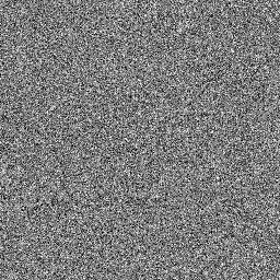 |
Mean = 125, $\sigma = 50$ | Depends on outliers | High ($\frac{50}{125} = 0.4$) | Very high (rapid changes) |
Key Insight: Luminance contrast suggests images A and B are identical, but RMS and local contrast reveal their structural differences. Choose the metric that aligns with your application’s needs.
Applications in Computer Vision
1. Adaptive Contrast Enhancement
CLAHE (Contrast Limited Adaptive Histogram Equalization) uses local contrast to decide where to enhance:
import cv2

# Compute local contrast map
local_contrast_map = local_contrast(image)

# Limit enhancement in already high-contrast regions
clahe = cv2.createCLAHE(clipLimit=2.0, tileGridSize=(8, 8))
enhanced = clahe.apply(image)
Why it works: High local contrast often means edges or texture—enhancing further just amplifies noise. Low local contrast suggests flat regions where boosting reveals hidden detail.
2. Exposure Fusion
When merging multiple exposures (HDR to SDR), preserve regions with high local contrast from the best-exposed image:
\[w_i(x, y) = C_{\text{local}, i}(x, y) \cdot S_i(x, y) \cdot E_i(x, y)\]where:
- $C_{\text{local}, i}$ = local contrast weight
- $S_i$ = saturation weight
- $E_i$ = well-exposedness weight
The final fused image is a weighted blend that prioritizes high-contrast, well-exposed regions.
3. Image Quality Assessment
Metrics like BRISQUE (Blind/Referenceless Image Spatial Quality Evaluator) use local contrast statistics to predict perceptual quality:
- Natural images have characteristic local contrast distributions
- Distorted images (compression artifacts, blur, noise) deviate from these distributions
- Machine learning models trained on local contrast features can predict MOS (Mean Opinion Score)
4. Retinal Image Analysis
In medical imaging, contrast-to-noise ratio (CNR) combines contrast with noise assessment:
\[\text{CNR} = \frac{\mid \mu_{\text{lesion}} - \mu_{\text{background}} \mid}{\sigma_{\text{background}}}\]High CNR means the lesion is easily distinguishable from the background, critical for automated diagnosis.
Choosing the Right Contrast Metric
| Metric | Best For | Limitations |
|---|---|---|
| Luminance Contrast | Quick global assessment, histogram decisions | Ignores spatial structure, outlier-prone |
| Michelson Contrast | Periodic patterns, MTF testing, display calibration | Requires clear peaks and troughs |
| RMS Contrast | Statistical analysis, global variation measure | Conflates magnitude and spatial frequency |
| Local Contrast | Adaptive processing, texture analysis, edge preservation | Computationally expensive, window-size dependent |
| Weber Contrast | Perceptual salience, legibility against backgrounds | Undefined for zero background, target-dependent |
| CSF-Weighted | Perceptual quality metrics, lossy compression | Requires multi-scale analysis, complex to implement |
Implementation Tips
1. Normalize Before Comparing
Contrast metrics often assume a specific intensity range. Always normalize to ([0, 1]) or your metric’s expected domain.
2. Handle Edge Cases
- Division by zero: Add a small epsilon ((\epsilon = 10^{-10})) to denominators
- Negative contrasts: Some formulations (Weber) can go negative; decide if you want absolute values
- Clipping: Ensure computed contrasts stay within valid ranges
3. Choose Window Size Carefully
For local contrast:
- Small windows (3×3, 5×5): Capture fine detail, sensitive to noise
- Large windows (15×15, 31×31): Smooth over noise, miss fine textures
- Adaptive sizing: Scale window based on local frequency content (expensive but accurate)
4. Combine Metrics
No single metric tells the whole story. Consider a contrast feature vector:
\[\mathbf{f}_{\text{contrast}} = [C_{\text{luminance}}, C_{\text{RMS}}, \text{mean}(C_{\text{local}}), \text{std}(C_{\text{local}}), \text{entropy}(I)]\]Use this vector for machine learning-based quality assessment or content-adaptive processing.
Contrast in Color Images
All the above definitions extend to color in two main ways:
1. Luminance-Only
Convert to grayscale (perceptually weighted):
\[Y = 0.299R + 0.587G + 0.114B\]Then apply any contrast metric to (Y). Advantage: Simple, perceptually meaningful. Disadvantage: Ignores chromatic contrast.
2. Per-Channel or Multi-Dimensional
Compute contrast in each RGB channel separately, then combine:
\[C_{\text{color}} = \sqrt{C_R^2 + C_G^2 + C_B^2}\]Or work in perceptual spaces like Lab:
\[C_{\text{Lab}} = \sqrt{(\Delta L^*)^2 + (\Delta a^*)^2 + (\Delta b^*)^2}\]Use case: Detecting colored patterns on colored backgrounds where luminance contrast is weak but chromatic contrast is strong.
Conclusion: Contrast Is Not One Thing
Image contrast is a family of related concepts, not a single definition. When someone says “increase the contrast,” they could mean:
- Stretching the histogram (luminance contrast)
- Enhancing edges (local contrast)
- Boosting high-frequency detail (CSF-weighted)
- Making features pop against backgrounds (Weber contrast)
Understanding these distinctions helps you:
- Choose the right metric for quality assessment or adaptive processing
- Interpret results when debugging vision algorithms
- Communicate precisely with colleagues about image properties
The next time you encounter a “low-contrast” image, ask: low by which measure? The answer will guide your enhancement strategy and set realistic expectations for what’s recoverable.
Further Reading
- Peli, E. (1990). “Contrast in complex images.” Journal of the Optical Society of America A, 7(10), 2032-2040.
- Barten, P. G. J. (1999). Contrast Sensitivity of the Human Eye and Its Effects on Image Quality. SPIE Press.
- Reinhard, E. et al. (2010). High Dynamic Range Imaging: Acquisition, Display, and Image-Based Lighting. Morgan Kaufmann.
- Mittal, A. et al. (2012). “No-Reference Image Quality Assessment in the Spatial Domain.” IEEE Transactions on Image Processing, 21(12), 4695-4708.
Have you encountered a computer vision problem where choosing the right contrast metric made a difference? Share your experience in the comments or reach out—I’d love to hear how these concepts play out in practice.